BANA6043: SAS Summary Stats
Matt Risley
Week 1 Lecture Series
1 Intro
SAS makes summary statistics fairly simple. The following are the most common ways to generate data and statistical summaries:
- PROC FREQ
- generates table of frequencies of values for a particular variable
- can answer the question, “how many?”
- useful for categorical variables
- PROC MEANS
- provides basic descriptive statistics such as mean, standard deviation, minimum and maximum
- useful for continuous variables
- PROC UNIVARIATE
- provides more detailed descriptive statistics than PROC MEANS
2 PROC FREQ
The SAS document is here.
Frequency tables answer the question, “how many?”
For example, in a data set of cars, you may ask, “how many cars are blue?” PROC FREQ will give you this information, as well as counts for all other colors.
Let’s see how PROC FREQ works with a data set of car evaluations.
2.1 Car Evaluation Data Description
The data set is sourced from the UCI Machine Learning Repository.
The target variable is vehicle “quality”, which has the variable name “class” in the data set.
There are several explanatory variables, including price and safety.
2.2 PROC FREQ Example
We can run a frequency table on all variables in the data set through the following code:
proc freq data=mrrlib.car_eval;
run;Note that all explanatory variables have the same frequency, but vehicle quality is not evenly distributed. This data set is output from a hierarchical decision model. Interactions among the explanatory variables ultimately inform the vehicle quality.
If we just wanted to see the frequency table for the target variable, we can use the tables statement:
proc freq data=mrrlib.car_eval;
tables class;
run;
On the surface, the data set and PROC FREQ output seem pretty boring. However, PROC FREQ can be powerful when evaluating two-way frequencies.
Of all the variables, suppose we assume that safety is a primary determinant of vehicle quality. After all, most drivers don’t particularly like an unsafe car.
We can run a two-way frequency table on class and safety. We simply use the asterisk symbol (*) between the two variables:
proc freq data=mrrlib.car_eval;
tables class*safety;
run;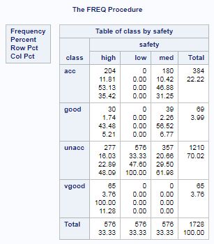
We can see that only unacceptable quality cars have a safety rating of low and that only very good quality cars have a safety rating of high.
2.3 PROC FREQ with Options
The code below specifies options for the tables statement. Options of this sort require a forward slash (/). These options return: (1) the Pearson chi-square coefficient and associated p-value as well as (2) a two-way frequency plot.
proc freq data=mrrlib.car_eval;
tables class*safety /
    chisq plots(only)=freqplot(twoway=cluster);
run;As shown in the output, there is evidence of an association between safety and quality.
You can also do a three-way (or more) frequency. These become somewhat difficult to read, however. They can sometimes be useful when the variables include some binary data.
3 PROC MEANS
The SAS document is here.
PROC MEANS provides the following descriptive statistics for a distribution of values:
- Measures of location
- mean
- median
- mode
- Measures of spread
- range
- percentiles
- standard deviation and variance
- Measures of shape
- kurtosis, skewness
It can also provide other information, such as confidence intervals.
Let’s see how PROC FREQ works with the Morley data set.
3.1 Morley Data Description
The Morley data set represents measurements of the speed of light from an 1879 experiment. The data include three variables: (1) experiment number, (2) run number, and (3) the measured speed. 5 experiments were conducted, each with 20 runs (or observations). See the R document for more information.
3.2 PROC MEANS Example
Because descriptive statistics do not make much sense for the experiment and run numbers, we will limit output only for the speed variable through the var statement.
proc means data=mrrlib.morley;
    var speed;
run;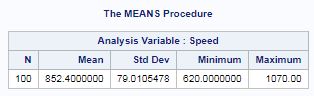
We can see that for the 100 runs, the average speed of light was 852.4 km/sec with a range of 620 to 1070 km/sec.
3.3 PROC MEANS with Options
What if we want to output summary statistics for each of the five experiments? We can use the BY statement, as shown in the code below.
In addition, we can add options to the PROC. The maxdec option limits the number of decimals to display in output, while “n mean median mode …” provide specified statistical measures other than the default. In this example, the CLM option provides a 95% confidence interval for the mean. If we wanted a 90% CI, we’d change alpha to 0.10.
proc means data=mrrlib.morley maxdec=1
n mean clm alpha=0.05 median mode min max skewness;
    var speed;
    by expt;
run;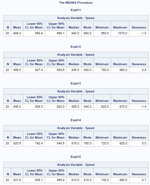
4 PROC UNIVARIATE
The SAS document is here.
PROC UNIVARIATE provides a variety of statistics for a supplied variable. PROC UNIVARIATE is useful when you need more sophistical statistical output such as:
- tests for normality
- outlier analysis
- trimmed/Winsorized means, which account for outliers
- confidence intervals around the standard deviation and quantiles
We’ll use the Morley data set again to demonstrate PROC UNIVARIATE.
4.1 PROC UNIVARIATE Example
The below code produces the default output, which includes a summary of moments, basic measures, tests for location, quantiles, and extreme observations.
proc univariate data=mrrlib.morley;
    var speed;
run;Note: the test of location are against a null of a mean of zero, which is not very intuitive.
4.2 PROC UNIVARIATE with Options
4.2.1 Histogram
proc univariate data=mrrlib.morley noprint;
    histogram speed / midpoints=uniform;
    class expt;
    inset mean="Mean Speed" / position=ne;
    label expt="Experiment Number";
run;The code above has the following features:
- calls the noprint option in the PROC in order to supress the default output shown above
- uses the HISTOGRAM statement with the midpoints=uniform option, which creates a uniform number of bins for all plots
- uses the CLASS statement to produce the output for each experiment
- instead of the BY statement, the CLASS statement is used to ensure all x-axes have the same range
- uses the INSET statement to create a legend with the mean for every experiment
- the position=ne option places the legend in the “northeast” (top right) corner
- uses the expt variable as label
4.2.2 Normality Testing
ods graphics on;
ods select Moments TestsForNormality ProbPlot;
proc univariate data=mrrlib.morley normaltest;
   var speed;
   by expt;
   probplot speed / normal (mu=est sigma=est)
                        square;
   label expt = 'Experiment Number' speed="Speed";
   inset  mean std / format=6.4;
run;The code above has the following features:
- turns on ODS Graphics, which creates high quality graphical output
- uses the ods select statement to only include Moments, TestsForNormality, and ProbPlot from PROC UNIVARIATE in the output
- uses the normaltest option to display tests for normality
- uses the by statement to produce the output for each experiment
- uses the probplot statement to create probability plots, which are similar to Q-Q plots
- the normal option requests a reference line of a normal distribution with a mean and standard deviation
- (mu=est sigma=est) requests the reference line to have the same mean and standard deviation as the sample
- square requests the plot be in the shape of a square
- uses the LABEL statement to create labels
- uses the INSET statement to include a legend with mean and standard deviation
- the format option specifies max place values of 6 and max decimal places of 4
The data are normal when:
- skewness = 0 and kurtosis = 3
- the goodness-of-fit tests fail to reject the null hypothesis of normality
- the points on the probability plot are near-linear and align with the reference line
4.2.3 Testing Measures of Location
As noted above, the tests for location in PROC UNIVARIATE are by default a two-tailed hypothesis test against a null of a mean of zero.
In the Morley data set, the experiment records the speed of light in km/sec with 299,000 km/sec subtracted from the result.
The speed of light in a vaccuum, c, is 299,792,458 meters/sec. Let’s use SAS to determine whether the results of each experiment confirm this measurement.
ods graphics on;
ods select testsforlocation;
proc univariate data=mrrlib.morley
mu0=792.458;
    var speed;
    title "Two-Tailed Test against Mean of 792.5: All Runs";
run;

ods graphics on;
ods select testsforlocation;
proc univariate data=mrrlib.morley
location=792.458; /*location is equivalent to mu0*/
    var speed;
    class expt;
    title "Two-Tailed Test against Mean of 792.5: Each Experiment";
run;We test the hypothesis first against all 100 runs. We then test the hypothesis against each of the 5 experiments. The tests of location reject the hypothesis that the mean speed of light is 299,792.5 km/sec.
The code above has the following features:
- turns on ODS Graphics, which creates high quality graphical output
- uses the ods select statement to only include TestsforLocation
- uses the mu0 (location) option for PROC UNIVARIATE
- uses the global TITLE statement to label output
- stacks two PROC UNIVARIATE in the output
PROC UNIVARIATE only supports two-tailed tests against a mean. However, the PROC provides alternatives to Student’s t for data that are not normally distributed.